Bring Excel Data to Life with Conditional Formatting

Data that Tells a Story

OVERVIEW: Learn how to use Microsoft Excel 2007’s advanced conditional formatting features to take your boring data and make it tell a more interesting story.

Boring Data Be Gone!

Have you ever created a spreadsheet that tracks a lot of important data? This data may have a lot to say, if you help it. Excel 2007 has some advanced Conditional Formatting features that allow you to use the values in cells to create visually informative displays that add more useful context to your information.

Take a look at the spreadsheet below. It lists the amount of fruits sold on each day of the week. There are a lot of numbers there and it might be kind of hard to spot any useful trends.

Let’s take a look at how we can use conditional formatting to identify things like: the biggest selling items on any day, the top, middle, and bottom sellers, use color shadings to indicate where each product ranks.

Video Tutorial Showing How to Use Conditional Formatting in Excel

Play the video below to see all of the options in action.

How to Use Conditional Formatting in Excel from Christopher Masiello on Vimeo.

Accessing the Conditional Formatting Menu

Click the Conditional Formatting icon on the Home tab of the Excel Ribbon.

You will see a menu with a list of Conditional Formatting options.

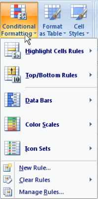
Let’s take a look at what these options can do.

Highlighting Cells with Specific Values

Click Conditional Formatting> Highlight Cell Rules> Greater Than.

A pop-up menu will open allowing you to enter the Greater Than amount and the formatting style.

In the example above, all cells whose value is greater than 500 were turned light red with dark red text. You can modify either of these settings. The other Highlight Cell Rules options work similarly.

Dynamically Highlighting Cells Using Top and Bottom Rules

You can highlight cells with values in the top or bottom “X” percent or “X” values in a range.

Click Conditional Formatting> Top/Bottom Rules> Top 10%.

A pop-up menu will open allowing you to enter the Percentage and the formatting style.

In the example below, the cells whose value is in the top 10% of the range were turned light red with dark red text. You can modify either of these settings. The other Top/Bottom Rules options work similarly.

Using Data Bars to Graphically Display Values

You can fill the cells in a range with data bars that are sized according their values.

Click Conditional Formatting> Data Bars and select a bar color.

Excel will find the highest and lowest values in the range and fill each cell accordingly with a colored bar.

Formatting the Cells in a Range Using Color Scales

You can use scales of color to highlight all of the cells in a range. You have a choice of shades of two or three colors.

Click Conditional Formatting> Color Scales and select your color set.

In the example below, the range of cell values were identified by the top, middle, and bottom thirds. The thirds were colored Red, Yellow, and Blue. Then, the values in each third were made darker or lighter depending on how close to the floor or ceiling of their ranges.

Identifying Cell Values Using Icons

The previous formatting option is often referred to as “stoplight” formatting (red, yellow, green). If you want to take it even more literally, you can place icons next to cell values.

Click Conditional Formatting> Icon Sets and select an icon type.

In the example below, the range of cell values were identified by the top, middle, and bottom thirds. The values in each third were identified by a red, yellow, or green icon.

There are several useful icons that you can use to identify your data set.

The other cool option that you can do is filter values based on their icon (meaning which section of the data range the values belong).

1. Go to theData tab
2. Click the Filter icon
3. Click the Filter Arrow at the top of the column that you want to filter
4. Select Filter by Color
5. Choose the icon that identifies the slice of the range that you want to filter on

You will see all of the values that have icon that you selected.

This is a pretty handy way to see the top sellers or worst performers in a range.